PyTorch一小时掌握之神经网络分类篇
概述
对于 MNIST 手写数据集的具体介绍, 我们在 TensorFlow 中已经详细描述过, 在这里就不多赘述. 有兴趣的同学可以去看看之前的文章: https://www.jb51.net/article/222183.htm
在上一节的内容里, 我们用 PyTorch 实现了回归任务, 在这一节里, 我们将使用 PyTorch 来解决分类任务.
导包
import torchvision
import torch
import torch.nn as nn
import torch.nn.functional as F
import torch.optim as optim
import matplotlib.pyplot as plt
设置超参数
# 设置超参数
n_epochs = 3
batch_size_train = 64
batch_size_test = 1000
learning_rate = 0.01
momentum = 0.5
log_interval = 10
random_seed = 1
torch.manual_seed(random_seed)
读取数据
# 数据读取
train_loader = torch.utils.data.DataLoader(
 torchvision.datasets.MNIST('./data/', train=True, download=True,
transform=torchvision.transforms.Compose([
 torchvision.transforms.ToTensor(),
 torchvision.transforms.Normalize(
  (0.1307,), (0.3081,))
])),
 batch_size=batch_size_train, shuffle=True)

test_loader = torch.utils.data.DataLoader(
 torchvision.datasets.MNIST('./data/', train=False, download=True,
transform=torchvision.transforms.Compose([
 torchvision.transforms.ToTensor(),
 torchvision.transforms.Normalize(
  (0.1307,), (0.3081,))
])),
 batch_size=batch_size_test, shuffle=True)
examples = enumerate(test_loader)
batch_idx, (example_data, example_targets) = next(examples)
# 调试输出
print(example_targets)
print(example_data.shape)
输出结果:
tensor([7, 6, 7, 5, 6, 7, 8, 1, 1, 2, 4, 1, 0, 8, 4, 4, 4, 9, 8, 1, 3, 3, 8, 6,
2, 7, 5, 1, 6, 5, 6, 2, 9, 2, 8, 4, 9, 4, 8, 6, 7, 7, 9, 8, 4, 9, 5, 3,
1, 0, 9, 1, 7, 3, 7, 0, 9, 2, 5, 1, 8, 9, 3, 7, 8, 4, 1, 9, 0, 3, 1, 2,
3, 6, 2, 9, 9, 0, 3, 8, 3, 0, 8, 8, 5, 3, 8, 2, 8, 5, 5, 7, 1, 5, 5, 1,
0, 9, 7, 5, 2, 0, 7, 6, 1, 2, 2, 7, 5, 4, 7, 3, 0, 6, 7, 5, 1, 7, 6, 7,
2, 1, 9, 1, 9, 2, 7, 6, 8, 8, 8, 4, 6, 0, 0, 2, 3, 0, 1, 7, 8, 7, 4, 1,
3, 8, 3, 5, 5, 9, 6, 0, 5, 3, 3, 9, 4, 0, 1, 9, 9, 1, 5, 6, 2, 0, 4, 7,
3, 5, 8, 8, 2, 5, 9, 5, 0, 7, 8, 9, 3, 8, 5, 3, 2, 4, 4, 6, 3, 0, 8, 2,
7, 0, 5, 2, 0, 6, 2, 6, 3, 6, 6, 7, 9, 3, 4, 1, 6, 2, 8, 4, 7, 7, 2, 7,
4, 2, 4, 9, 7, 7, 5, 9, 1, 3, 0, 4, 4, 8, 9, 6, 6, 5, 3, 3, 2, 3, 9, 1,
1, 4, 4, 8, 1, 5, 1, 8, 8, 0, 7, 5, 8, 4, 0, 0, 0, 6, 3, 0, 9, 0, 6, 6,
9, 8, 1, 2, 3, 7, 6, 1, 5, 9, 3, 9, 3, 2, 5, 9, 9, 5, 4, 9, 3, 9, 6, 0,
3, 3, 8, 3, 1, 4, 1, 4, 7, 3, 1, 6, 8, 4, 7, 7, 3, 3, 6, 1, 3, 2, 3, 5,
9, 9, 9, 2, 9, 0, 2, 7, 0, 7, 5, 0, 2, 6, 7, 3, 7, 1, 4, 6, 4, 0, 0, 3,
2, 1, 9, 3, 5, 5, 1, 6, 4, 7, 4, 6, 4, 4, 9, 7, 4, 1, 5, 4, 8, 7, 5, 9,
2, 9, 4, 0, 8, 7, 3, 4, 2, 7, 9, 4, 4, 0, 1, 4, 1, 2, 5, 2, 8, 5, 3, 9,
1, 3, 5, 1, 9, 5, 3, 6, 8, 1, 7, 9, 9, 9, 9, 9, 2, 3, 5, 1, 4, 2, 3, 1,
1, 3, 8, 2, 8, 1, 9, 2, 9, 0, 7, 3, 5, 8, 3, 7, 8, 5, 6, 4, 1, 9, 7, 1,
7, 1, 1, 8, 6, 7, 5, 6, 7, 4, 9, 5, 8, 6, 5, 6, 8, 4, 1, 0, 9, 1, 4, 3,
5, 1, 8, 7, 5, 4, 6, 6, 0, 2, 4, 2, 9, 5, 9, 8, 1, 4, 8, 1, 1, 6, 7, 5,
9, 1, 1, 7, 8, 7, 5, 5, 2, 6, 5, 8, 1, 0, 7, 2, 2, 4, 3, 9, 7, 3, 5, 7,
6, 9, 5, 9, 6, 5, 7, 2, 3, 7, 2, 9, 7, 4, 8, 4, 9, 3, 8, 7, 5, 0, 0, 3,
4, 3, 3, 6, 0, 1, 7, 7, 4, 6, 3, 0, 8, 0, 9, 8, 2, 4, 2, 9, 4, 9, 9, 9,
7, 7, 6, 8, 2, 4, 9, 3, 0, 4, 4, 1, 5, 7, 7, 6, 9, 7, 0, 2, 4, 2, 1, 4,
7, 4, 5, 1, 4, 7, 3, 1, 7, 6, 9, 0, 0, 7, 3, 6, 3, 3, 6, 5, 8, 1, 7, 1,
6, 1, 2, 3, 1, 6, 8, 8, 7, 4, 3, 7, 7, 1, 8, 9, 2, 6, 6, 6, 2, 8, 8, 1,
6, 0, 3, 0, 5, 1, 3, 2, 4, 1, 5, 5, 7, 3, 5, 6, 2, 1, 8, 0, 2, 0, 8, 4,
4, 5, 0, 0, 1, 5, 0, 7, 4, 0, 9, 2, 5, 7, 4, 0, 3, 7, 0, 3, 5, 1, 0, 6,
4, 7, 6, 4, 7, 0, 0, 5, 8, 2, 0, 6, 2, 4, 2, 3, 2, 7, 7, 6, 9, 8, 5, 9,
7, 1, 3, 4, 3, 1, 8, 0, 3, 0, 7, 4, 9, 0, 8, 1, 5, 7, 3, 2, 2, 0, 7, 3,
1, 8, 8, 2, 2, 6, 2, 7, 6, 6, 9, 4, 9, 3, 7, 0, 4, 6, 1, 9, 7, 4, 4, 5,
8, 2, 3, 2, 4, 9, 1, 9, 6, 7, 1, 2, 1, 1, 2, 6, 9, 7, 1, 0, 1, 4, 2, 7,
7, 8, 3, 2, 8, 2, 7, 6, 1, 1, 9, 1, 0, 9, 1, 3, 9, 3, 7, 6, 5, 6, 2, 0,
0, 3, 9, 4, 7, 3, 2, 9, 0, 9, 5, 2, 2, 4, 1, 6, 3, 4, 0, 1, 6, 9, 1, 7,
0, 8, 0, 0, 9, 8, 5, 9, 4, 4, 7, 1, 9, 0, 0, 2, 4, 3, 5, 0, 4, 0, 1, 0,
5, 8, 1, 8, 3, 3, 2, 1, 2, 6, 8, 2, 5, 3, 7, 9, 3, 6, 2, 2, 6, 2, 7, 7,
6, 1, 8, 0, 3, 5, 7, 5, 0, 8, 6, 7, 2, 4, 1, 4, 3, 7, 7, 2, 9, 3, 5, 5,
9, 4, 8, 7, 6, 7, 4, 9, 2, 7, 7, 1, 0, 7, 2, 8, 0, 3, 5, 4, 5, 1, 5, 7,
6, 7, 3, 5, 3, 4, 5, 3, 4, 3, 2, 3, 1, 7, 4, 4, 8, 5, 5, 3, 2, 2, 9, 5,
8, 2, 0, 6, 0, 7, 9, 9, 6, 1, 6, 6, 2, 3, 7, 4, 7, 5, 2, 9, 4, 2, 9, 0,
8, 1, 7, 5, 5, 7, 0, 5, 2, 9, 5, 2, 3, 4, 6, 0, 0, 2, 9, 2, 0, 5, 4, 8,
9, 0, 9, 1, 3, 4, 1, 8, 0, 0, 4, 0, 8, 5, 9, 8])
torch.Size([1000, 1, 28, 28])
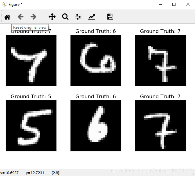
可视化展示
# 画图 (前6个)
fig = plt.figure()
for i in range(6):
 plt.subplot(2, 3, i + 1)
 plt.tight_layout()
 plt.imshow(example_data[i][0], cmap='gray', interpolation='none')
 plt.title("Ground Truth: {}".format(example_targets[i]))
 plt.xticks([])
 plt.yticks([])
plt.show()
输出结果:
建立模型
# 创建model
class Net(nn.Module):
 def __init__(self):
  super(Net, self).__init__()
  self.conv1 = nn.Conv2d(1, 10, kernel_size=5)
  self.conv2 = nn.Conv2d(10, 20, kernel_size=5)
  self.conv2_drop = nn.Dropout2d()
  self.fc1 = nn.Linear(320, 50)
  self.fc2 = nn.Linear(50, 10)
 def forward(self, x):
  x = F.relu(F.max_pool2d(self.conv1(x), 2))
  x = F.relu(F.max_pool2d(self.conv2_drop(self.conv2(x)), 2))
  x = x.view(-1, 320)
  x = F.relu(self.fc1(x))
  x = F.dropout(x, training=self.training)
  x = self.fc2(x)
  return F.log_softmax(x)

network = Net()
optimizer = optim.SGD(network.parameters(), lr=learning_rate,
 momentum=momentum)
训练模型
# 训练
train_losses = []
train_counter = []
test_losses = []
test_counter = [i * len(train_loader.dataset) for i in range(n_epochs + 1)]

def train(epoch):
 network.train()
 for batch_idx, (data, target) in enumerate(train_loader):
  optimizer.zero_grad()
  output = network(data)
  loss = F.nll_loss(output, target)
  loss.backward()
  optimizer.step()
  if batch_idx % log_interval == 0:
print('Train Epoch: {} [{}/{} ({:.0f}%)]\tLoss: {:.6f}'.format(
 epoch, batch_idx * len(data), len(train_loader.dataset),
  100. * batch_idx / len(train_loader), loss.item()))
train_losses.append(loss.item())
train_counter.append(
 (batch_idx * 64) + ((epoch - 1) * len(train_loader.dataset)))
torch.save(network.state_dict(), './model.pth')
torch.save(optimizer.state_dict(), './optimizer.pth')

def test():
 network.eval()
 test_loss = 0
 correct = 0
 with torch.no_grad():
  for data, target in test_loader:
output = network(data)
test_loss += F.nll_loss(output, target, size_average=False).item()
pred = output.data.max(1, keepdim=True)[1]
correct += pred.eq(target.data.view_as(pred)).sum()
 test_loss /= len(test_loader.dataset)
 test_losses.append(test_loss)
 print('\nTest set: Avg. loss: {:.4f}, Accuracy: {}/{} ({:.0f}%)\n'.format(
  test_loss, correct, len(test_loader.dataset),
  100. * correct / len(test_loader.dataset)))

for epoch in range(1, n_epochs + 1):
 train(epoch)
 test()
输出结果:
Train Epoch: 1 [0/60000 (0%)] Loss: 2.297471
Train Epoch: 1 [6400/60000 (11%)] Loss: 1.934886
Train Epoch: 1 [12800/60000 (21%)] Loss: 1.242982
Train Epoch: 1 [19200/60000 (32%)] Loss: 0.979296
Train Epoch: 1 [25600/60000 (43%)] Loss: 1.277279
Train Epoch: 1 [32000/60000 (53%)] Loss: 0.721533
Train Epoch: 1 [38400/60000 (64%)] Loss: 0.759595
Train Epoch: 1 [44800/60000 (75%)] Loss: 0.469635
Train Epoch: 1 [51200/60000 (85%)] Loss: 0.422614
Train Epoch: 1 [57600/60000 (96%)] Loss: 0.417603Test set: Avg. loss: 0.1988, Accuracy: 9431/10000 (94%)
Train Epoch: 2 [0/60000 (0%)] Loss: 0.277207
Train Epoch: 2 [6400/60000 (11%)] Loss: 0.328862
Train Epoch: 2 [12800/60000 (21%)] Loss: 0.396312
Train Epoch: 2 [19200/60000 (32%)] Loss: 0.301772
Train Epoch: 2 [25600/60000 (43%)] Loss: 0.253600
Train Epoch: 2 [32000/60000 (53%)] Loss: 0.217821
Train Epoch: 2 [38400/60000 (64%)] Loss: 0.395815
Train Epoch: 2 [44800/60000 (75%)] Loss: 0.265737
Train Epoch: 2 [51200/60000 (85%)] Loss: 0.323627
Train Epoch: 2 [57600/60000 (96%)] Loss: 0.236692Test set: Avg. loss: 0.1233, Accuracy: 9622/10000 (96%)
Train Epoch: 3 [0/60000 (0%)] Loss: 0.500148
Train Epoch: 3 [6400/60000 (11%)] Loss: 0.338118
Train Epoch: 3 [12800/60000 (21%)] Loss: 0.452308
Train Epoch: 3 [19200/60000 (32%)] Loss: 0.374940
Train Epoch: 3 [25600/60000 (43%)] Loss: 0.323300
Train Epoch: 3 [32000/60000 (53%)] Loss: 0.203830
Train Epoch: 3 [38400/60000 (64%)] Loss: 0.379557
Train Epoch: 3 [44800/60000 (75%)] Loss: 0.334822
Train Epoch: 3 [51200/60000 (85%)] Loss: 0.361676
Train Epoch: 3 [57600/60000 (96%)] Loss: 0.218833Test set: Avg. loss: 0.0911, Accuracy: 9723/10000 (97%)
完整代码
import torchvision
import torch
import torch.nn as nn
import torch.nn.functional as F
import torch.optim as optim
import matplotlib.pyplot as plt
# 设置超参数
n_epochs = 3
batch_size_train = 64
batch_size_test = 1000
learning_rate = 0.01
momentum = 0.5
log_interval = 100
random_seed = 1
torch.manual_seed(random_seed)
# 数据读取
train_loader = torch.utils.data.DataLoader(
 torchvision.datasets.MNIST('./data/', train=True, download=True,
transform=torchvision.transforms.Compose([
 torchvision.transforms.ToTensor(),
 torchvision.transforms.Normalize(
  (0.1307,), (0.3081,))
])),
 batch_size=batch_size_train, shuffle=True)
test_loader = torch.utils.data.DataLoader(
 torchvision.datasets.MNIST('./data/', train=False, download=True,
transform=torchvision.transforms.Compose([
 torchvision.transforms.ToTensor(),
 torchvision.transforms.Normalize(
  (0.1307,), (0.3081,))
])),
 batch_size=batch_size_test, shuffle=True)
examples = enumerate(test_loader)
batch_idx, (example_data, example_targets) = next(examples)
# 调试输出
print(example_targets)
print(example_data.shape)
# 画图 (前6个)
fig = plt.figure()
for i in range(6):
 plt.subplot(2, 3, i + 1)
 plt.tight_layout()
 plt.imshow(example_data[i][0], cmap='gray', interpolation='none')
 plt.title("Ground Truth: {}".format(example_targets[i]))
 plt.xticks([])
 plt.yticks([])
plt.show()

# 创建model
class Net(nn.Module):
 def __init__(self):
  super(Net, self).__init__()
  self.conv1 = nn.Conv2d(1, 10, kernel_size=5)
  self.conv2 = nn.Conv2d(10, 20, kernel_size=5)
  self.conv2_drop = nn.Dropout2d()
  self.fc1 = nn.Linear(320, 50)
  self.fc2 = nn.Linear(50, 10)
 def forward(self, x):
  x = F.relu(F.max_pool2d(self.conv1(x), 2))
  x = F.relu(F.max_pool2d(self.conv2_drop(self.conv2(x)), 2))
  x = x.view(-1, 320)
  x = F.relu(self.fc1(x))
  x = F.dropout(x, training=self.training)
  x = self.fc2(x)
  return F.log_softmax(x)

network = Net()
optimizer = optim.SGD(network.parameters(), lr=learning_rate,
 momentum=momentum)
# 训练
train_losses = []
train_counter = []
test_losses = []
test_counter = [i * len(train_loader.dataset) for i in range(n_epochs + 1)]

def train(epoch):
 network.train()
 for batch_idx, (data, target) in enumerate(train_loader):
  optimizer.zero_grad()
  output = network(data)
  loss = F.nll_loss(output, target)
  loss.backward()
  optimizer.step()
  if batch_idx % log_interval == 0:
print('Train Epoch: {} [{}/{} ({:.0f}%)]\tLoss: {:.6f}'.format(
 epoch, batch_idx * len(data), len(train_loader.dataset),
  100. * batch_idx / len(train_loader), loss.item()))
train_losses.append(loss.item())
train_counter.append(
 (batch_idx * 64) + ((epoch - 1) * len(train_loader.dataset)))
torch.save(network.state_dict(), './model.pth')
torch.save(optimizer.state_dict(), './optimizer.pth')

def test():
 network.eval()
 test_loss = 0
 correct = 0
 with torch.no_grad():
  for data, target in test_loader:
output = network(data)
test_loss += F.nll_loss(output, target, size_average=False).item()
pred = output.data.max(1, keepdim=True)[1]
correct += pred.eq(target.data.view_as(pred)).sum()
 test_loss /= len(test_loader.dataset)
 test_losses.append(test_loss)
 print('\nTest set: Avg. loss: {:.4f}, Accuracy: {}/{} ({:.0f}%)\n'.format(
  test_loss, correct, len(test_loader.dataset),
  100. * correct / len(test_loader.dataset)))

for epoch in range(1, n_epochs + 1):
 train(epoch)
 test()
到此这篇关于PyTorch一小时掌握之神经网络分类篇的文章就介绍到这了,更多相关PyTorch神经网络分类内容请搜索本站以前的文章或继续浏览下面的相关文章希望大家以后多多支持本站!
版权声明:本站文章来源标注为YINGSOO的内容版权均为本站所有,欢迎引用、转载,请保持原文完整并注明来源及原文链接。禁止复制或仿造本网站,禁止在非www.yingsoo.com所属的服务器上建立镜像,否则将依法追究法律责任。本站部分内容来源于网友推荐、互联网收集整理而来,仅供学习参考,不代表本站立场,如有内容涉嫌侵权,请联系alex-e#qq.com处理。
 关注官方微信