python光学仿真通过菲涅耳公式实现波动模型(光学波动)

从物理学的机制出发，波动模型相对于光线模型，显然更加接近光的本质；但是从物理学的发展来说，波动光学旨在解决几何光学无法解决的问题，可谓光线模型的一种升级。从编程的角度来说，波动光学在某些情况下可以简单地理解为在光线模型的基础上，引入一个相位项。

波动模型

一般来说，三个特征可以确定空间中的波场：频率、振幅和相位，故光波场可表示为：

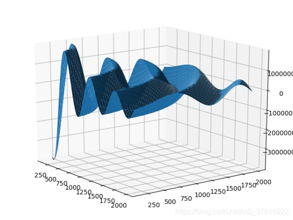
import numpy as np
import matplotlib.pyplot as plt
from mpl_toolkits.mplot3d import Axes3D
z = np.arange(15,200)*10 #单位为nm
x = np.arange(15,200)*10
x,z = np.meshgrid(x,z)#创建坐标系
E = 1/np.sqrt(x**2+z**2)*np.cos(2*np.pi*np.sqrt(x**2+z**2)/(532*1e-9))
fig = plt.figure()
ax = Axes3D(fig)
ax.plot_surface(x,z,E)
plt.show()

其结果如图所示

菲涅耳公式

几何光学可以通过费马原理得到折射定律，但是无法获知光波的透过率，菲涅耳公式在几何光学的基础上，解决了这个问题。

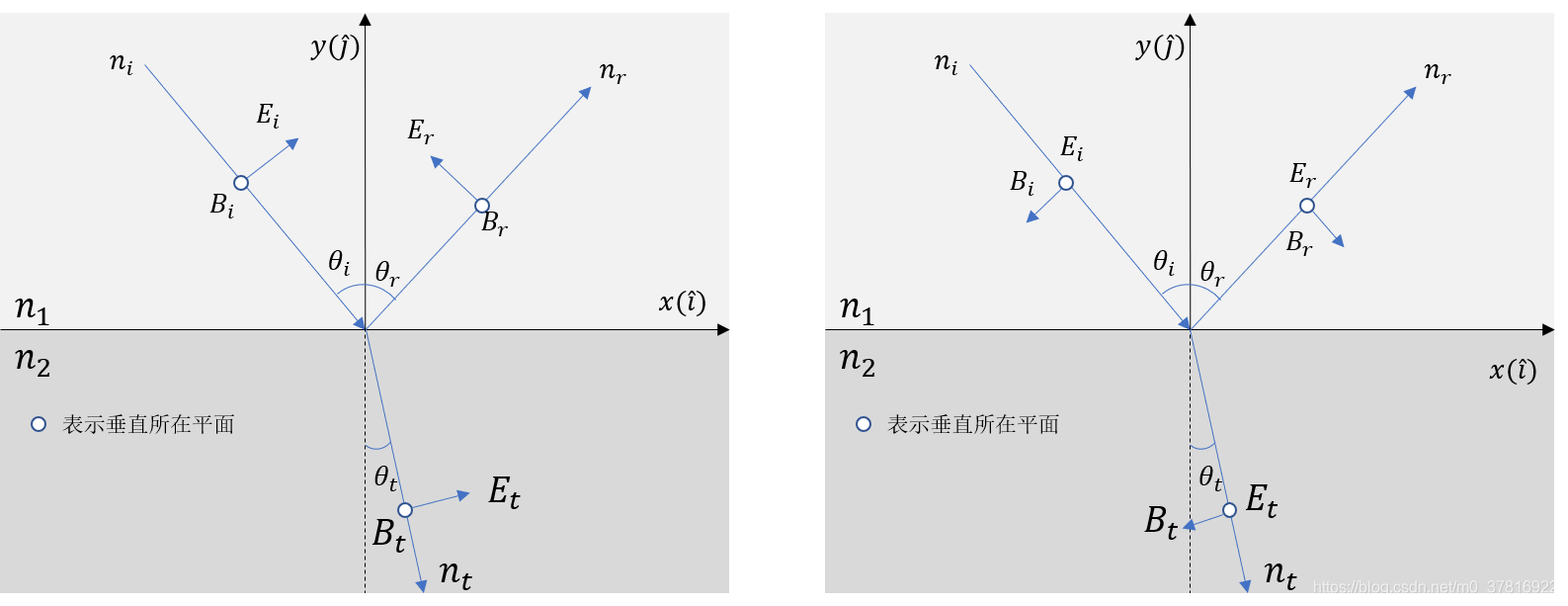
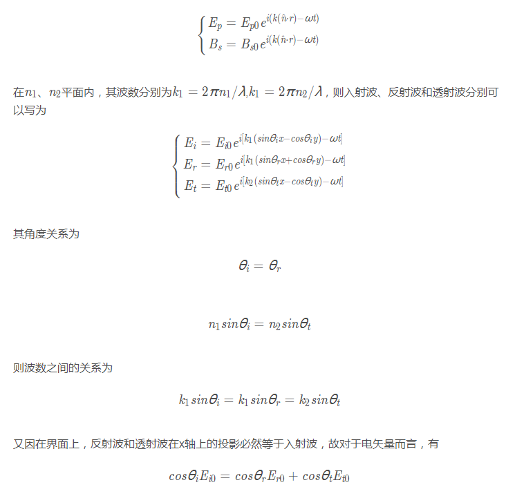
由于光是一群横波的集合，故可以根据其电矢量的震动方向，将其分为平行入射面与垂直入射面的两个分量，分别用p分量和 s 分量来表示。一束光在两介质交界处发生折射，两介质折射率分别为 n1和 n2，对于 p光来说，其电矢量平行于入射面，其磁矢量则垂直于入射面，即只有s分量；而对于 s光来说，则恰恰相反，如图所示。

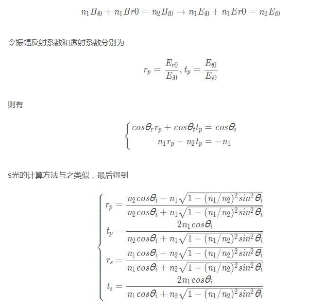
则对于 p 光来说即

对于磁矢量而言，有

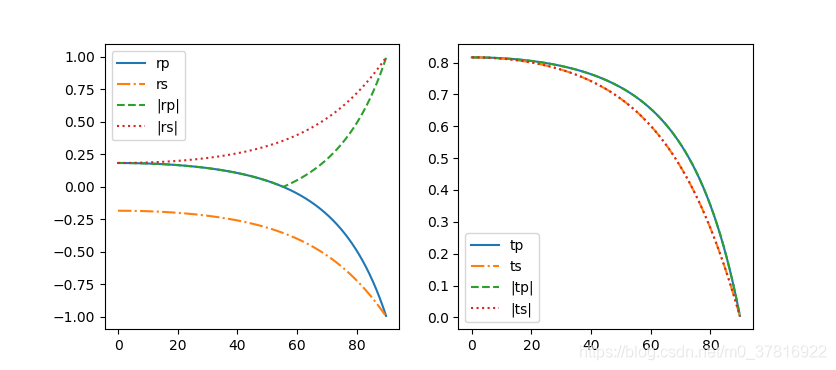
我们可以通过python绘制出当入射光的角度不同时，其振幅反射率和透过率的变化

import matplotlib.pyplot as plt
import numpy as np
def fresnel(theta, n1, n2):
 theta = theta*np.pi/180
 xTheta = np.cos(theta)
 mid = np.sqrt(1-(n1/n2*np.sin(theta))**2) #中间变量
 rp = (n2*xTheta-n1*mid)/(n2*xTheta+n1*mid)  #p分量振幅反射率
 rs = (n1*xTheta-n2*mid)/(n1*xTheta+n2*mid)
 tp = 2*n1*xTheta/(n2*xTheta+n1*mid)
 ts = 2*n1*xTheta/(n1*xTheta+n2*mid)
 return rp, rs, tp, ts
def testFres(n1=1,n2=1.45):#默认n2为1.45
 theta = np.arange(0,90,0.1)+0j
 a = theta*np.pi/180
 rp,rs,tp,ts = fresnel(theta,n1,n2)
 fig = plt.figure(1)
 plt.subplot(1,2,1)
 plt.plot(theta,rp,'-',label='rp')
 plt.plot(theta,rs,'-.',label='rs')
 plt.plot(theta,np.abs(rp),'--',label='|rp|')
 plt.plot(theta,np.abs(rs),':',label='|rs|')
 plt.legend()
 plt.subplot(1,2,2)
 plt.plot(theta,tp,'-',label='tp')
 plt.plot(theta,ts,'-.',label='ts')
 plt.plot(theta,np.abs(tp),'--',label='|tp|')
 plt.plot(theta,np.abs(ts),':',label='|ts|')
 plt.legend()
 plt.show()
if __init__=="__main__":
 testFres()

得到其图像为

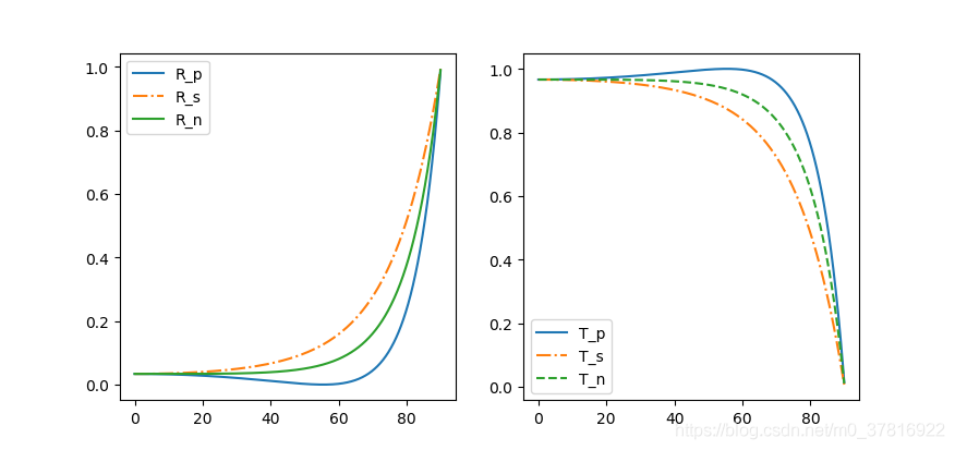
通过python进行绘图，将上面程序中的testFres改为以下代码即可。

def testFres(n1=1,n2=1.45):
 theta = np.arange(0,90,0.1)+0j
 a = theta*np.pi/180
 rp,rs,tp,ts = fml.fresnel(theta,n1,n2)
 Rp = np.abs(rp)**2
 Rs = np.abs(rs)**2
 Rn = (Rp+Rs)/2
 Tp = n2*np.sqrt(1-(n1/n2*np.sin(a))**2)/(n1*np.cos(a))*np.abs(tp)**2
 Ts = n2*np.sqrt(1-(n1/n2*np.sin(a))**2)/(n1*np.cos(a))*np.abs(ts)**2
 Tn = (Tp+Ts)/2
 fig = plt.figure(2)
 plt.subplot(1,2,1)
 plt.plot(theta,Rp,'-',label='R_p')
 plt.plot(theta,Rs,'-.',label='R_s')
 plt.plot(theta,Rn,'-',label='R_n')
 plt.legend()
 plt.subplot(1,2,2)
 plt.plot(theta,Tp,'-',label='T_p')
 plt.plot(theta,Ts,'-.',label='T_s')
 plt.plot(theta,Tn,'--',label='T_n')
 plt.legend()
 plt.show()

得